Also called theme rivers and in some cases steam graphs.
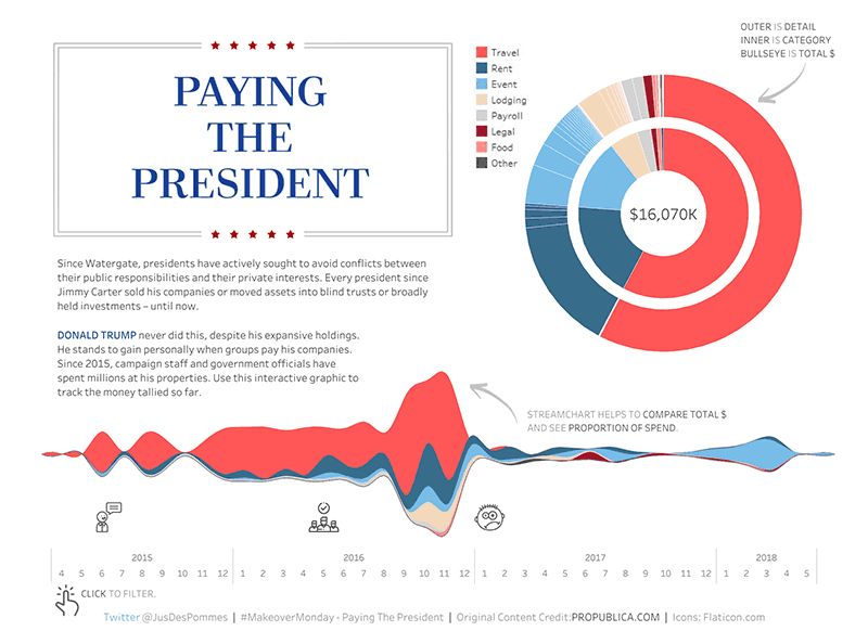
It all started with this viz by Alex Jones:
From the moment I saw it, I knew I wanted to create one by myself.
Fortunately, Alex offered some insights on how he did it, but he didn’t give up the whole thing.
Reverse engineering is probably my favorite part of the work, so rock on!
Before we start
If you want to dig in further on stream graphs, Andy Kirk has a fantastic post way back from 2010. He offers examples, opinions, and advice to get the best out of this type of charts.
It’s clear that stacking up areas makes them difficult to compare amongst each other. To make it even more difficult, we are going to use smooth lines instead of straight ones.
Curvy lines, you guessed it, are not best practice!
For me, a streamgraph is an aesthetically pleasing visualization that offers a different approach to stacked area charts.
There are many alternatives of course. However, I saw this as an exciting challenge and an excellent opportunity to learn something new.
With that out of the way let’s dig in!
Starting up
We will do most of the heavy lifting in R and export the data into Tableau to build the visualization using polygons.
Getting the data ready
Let’s start with an air pollution dataset I got from the European Environment Agency.
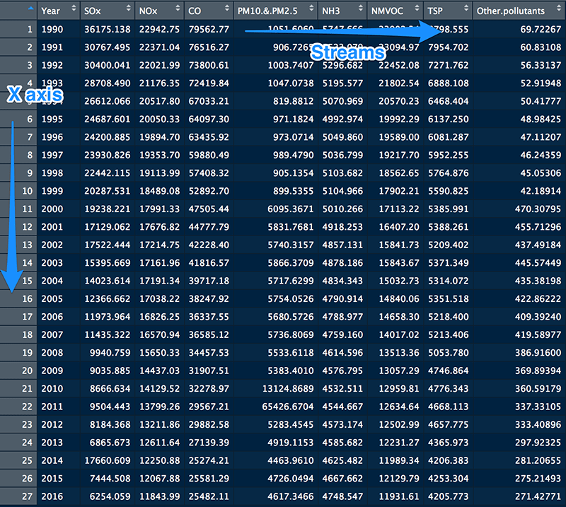
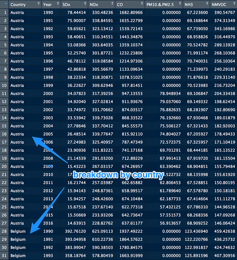
I grouped and pivoted the data to have a row for each element on the X-axis (in our case Year) and a column for each stream (in our case pollutant):
If your data is missing some values, you can replace those with 0.
Here comes the R code
Pay close attention to the comments in the code. In some cases, you will need to change the values to fit your particular case.
The code is heavily based on Paolo Toffanin’s work on how to build stream graphs in base R.
##function that implements the ThemeRiver and Zero Value algorithms
computeStacks <- function(values, method = "ThemeRiver"){
  timePoints <- dim(values)[1]
  nStreams <- dim(values)[2]
  yy <- matrix(0, timePoints, (nStreams * 2))
  for (iStream in 1 : nStreams){
    tmpVals <- values[, iStream]
    if (iStream > 1){
      yy[, iStream * 2 - 1] <- yy[, (iStream - 1) * 2]
      yy[, iStream * 2] <- yy[, iStream * 2 - 1] + tmpVals
    } else {
      switch(method,
             ThemeRiver = {
               yy[, 1] <- -(1/2) * rowSums(values)
               yy[, 2] <- yy[, iStream * 2 - 1] + tmpVals},
             zero = {
               yy[, 2] <- tmpVals},
             { # default (no method selected)
               print(paste0(baseline, "not recognized"))
               print("algorithm can be zero or ThemeRiver")}
      )
    }# end: if (iStream > 1){
  }# end:
  return(yy)
}

##similar compute function; this version uses curved lines
computeSmoothedStacks <- function(values, method = "ThemeRiver",multiple){
  timePoints <- dim(values)[1]*multiple #the "multiple" is used to densify the data; higher values make the curves smoother, but they can increase the size of the data significantly
  nStreams <- dim(values)[2]
  yy <- matrix(0, timePoints, (nStreams * 2))
  for (iStream in 1 : nStreams){
    tmpVals <- spline(values[, iStream],n=timePoints)$y
    if (iStream > 1){
      yy[, iStream * 2 - 1] <- yy[, (iStream - 1) * 2]
      yy[, iStream * 2] <- yy[, iStream * 2 - 1] + tmpVals
    } else {
      switch(method,
             ThemeRiver = {
               yy[, 1] <- -(1/2) * spline(rowSums(values),n=timePoints)$y
               yy[, 2] <- yy[, iStream * 2 - 1] + tmpVals},
             zero = {
               yy[, 2] <- tmpVals},
             { # default
               print(paste0(baseline, "not recognized"))
               print("algorithm can be zero or ThemeRiver")}
      )
    }# end: if (iStream > 1){
  }# end:
  return(yy)
}

##the following function plots the streamgraph and returns the coordinates to be exported
streamGraph <- function(yy, cols, plotTitle = "Streamgraph", streamNames=c()){
  timePoints <- dim(yy)[1]
  nStreams <- dim(yy)[2] / 2

  poly <- data.frame(Country = character(), x = numeric(), y = numeric(),col=character()) #initialize dataframe (used to grab the coordinates from the streamgraph)

  xx <- c(1:timePoints, timePoints:1)
  plot (xx, xx, type = "n", main = plotTitle,
        xlab = "Time",
        ylab = "Amplitude", ylim = range(yy),
        bty = "n")
  for (iStream in 1 : nStreams)
  {
    y <- c(yy[, iStream * 2], rev(yy[, iStream * 2 - 1]))
    polygon(xx, y, col = cols[iStream], border = NA)

    #take the data out
    poly <- rbind(poly,cbind(plotTitle,xx,y,streamNames[iStream]))
  }
  #return the line coordinates
  return(poly)
}

#read the data from an Excel file
library(openxlsx)
setwd("~/Downloads/")
pol <- read.xlsx("pollution-agg.xlsx")

#clean the data
pol$Year <- NULL #we have to clear the X-axis field; if it's name is different in your case, make sure to change it accordingly
pol[is.na(pol)] <- 0
pol <- data.matrix(pol)
values <- pol
pollutants <- colnames(values)

#generate the color palette for the streams
colorPalette <- colorRampPalette(c("#436382", "#ec7181", "#b1bdc1"), space = "rgb") #you can update the color codes according to your needs (not needed for the Tableau visualization)
cols <- colorPalette(ncol(values))

##plot the graphs in R to double check if everything works (not needed for the Tableau visualization)
par(mfrow = c(2, 2))
#plot the straight-line stream graphs
streamGraph(computeStacks(values,method = "zero"), cols, "Zero Baseline")
streamGraph(computeStacks(values,method = "ThemeRiver"), cols, "Theme river")
#plot the smooth stream graphs
streamGraph(computeSmoothedStacks(values,multiple=15,method = "zero"), cols, "Smooth Zero Baseline")
streamGraph(computeSmoothedStacks(values,multiple=15,method = "ThemeRiver"), cols, "Smooth Theme River")
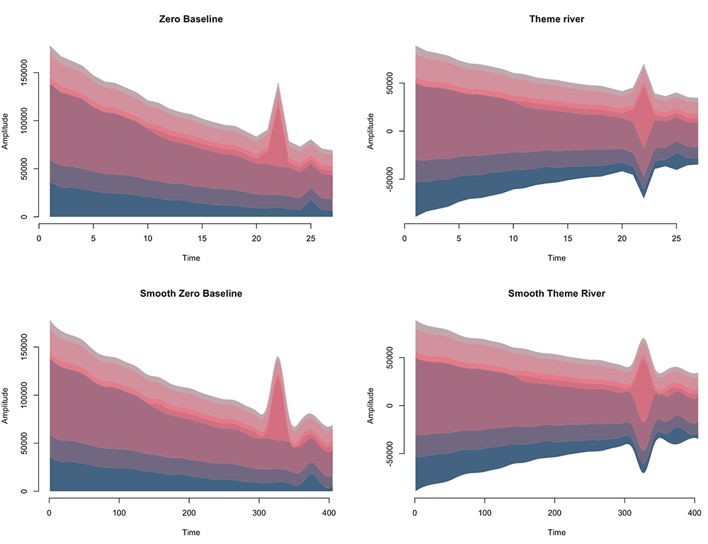
If everything works ok, you should be able to compare these different types of streamgraphs in the “Plots” window:
Now you can choose your preferred version and use the following code to get the coordinates data into a CSV file:
#take the data out of the streamgraph into a CSV file
streamNames <- colnames(values)
agg <- streamGraph(computeSmoothedStacks(values,multiple=15), cols, NULL, streamNames)
colnames(agg) <- c("X","Y","Pollutant")
agg$ID <- seq.int(nrow(agg)) #add consecutive IDs for the rows (to be used as Path in Tableau)
write.csv(agg,file="eu-stream.csv",row.names=F)
The Tableau part
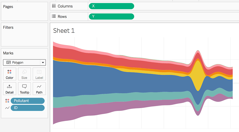
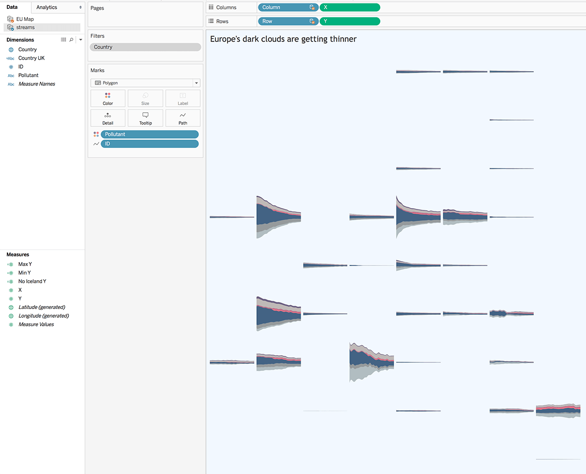
From here you just add the CSV into Tableau, and you place the fields like in the following screenshot:
Cool beans!
How about if we amp up the difficulty a bit?
Small Multiples
Let’s say you want to build a panel of stream charts. Well, we can build them one by one using a for loop in R.
All we have to do is to add the field we want to use for the breakdown inside the dataset (in our case Country):
In this case the R code used to build the stream graphs would look like this (all of our functions remain the same as above):
##small multiples
#read and clean the data
pol <- read.xlsx("pollution.xlsx")
library(tidyverse)
pol <- pol %>% fill(Country)
pol[is.na(pol)] <- 0

#plot the small multiples
par(mfrow = c(7, 5))
pi  <- data.frame(Country = character(), x = numeric(), y = numeric()); #initialize dataframe used to extract the data
for (country in unique(pol$Country)) {
  p <- pol[pol$Country==country,]
  p$Year <- NULL
  p$Country <- NULL
  p[is.na(p)] <- 0
  p <- data.matrix(p)
  values <- p
  cols <- colorPalette(ncol(values))
  pollutants <- colnames(values)
  tmp <- streamGraph(computeSmoothedStacks(values,multiple=5), cols, country, pollutants)
  pi <- rbind(pi,tmp) #fill up the dataframe with each of the small multiples
}
#take the data out into a CSV
colnames(pi) <- c("Country","X","Y","Pollutant")
pi$ID <- seq.int(nrow(pi))
write.csv(pi,file="streams.csv")
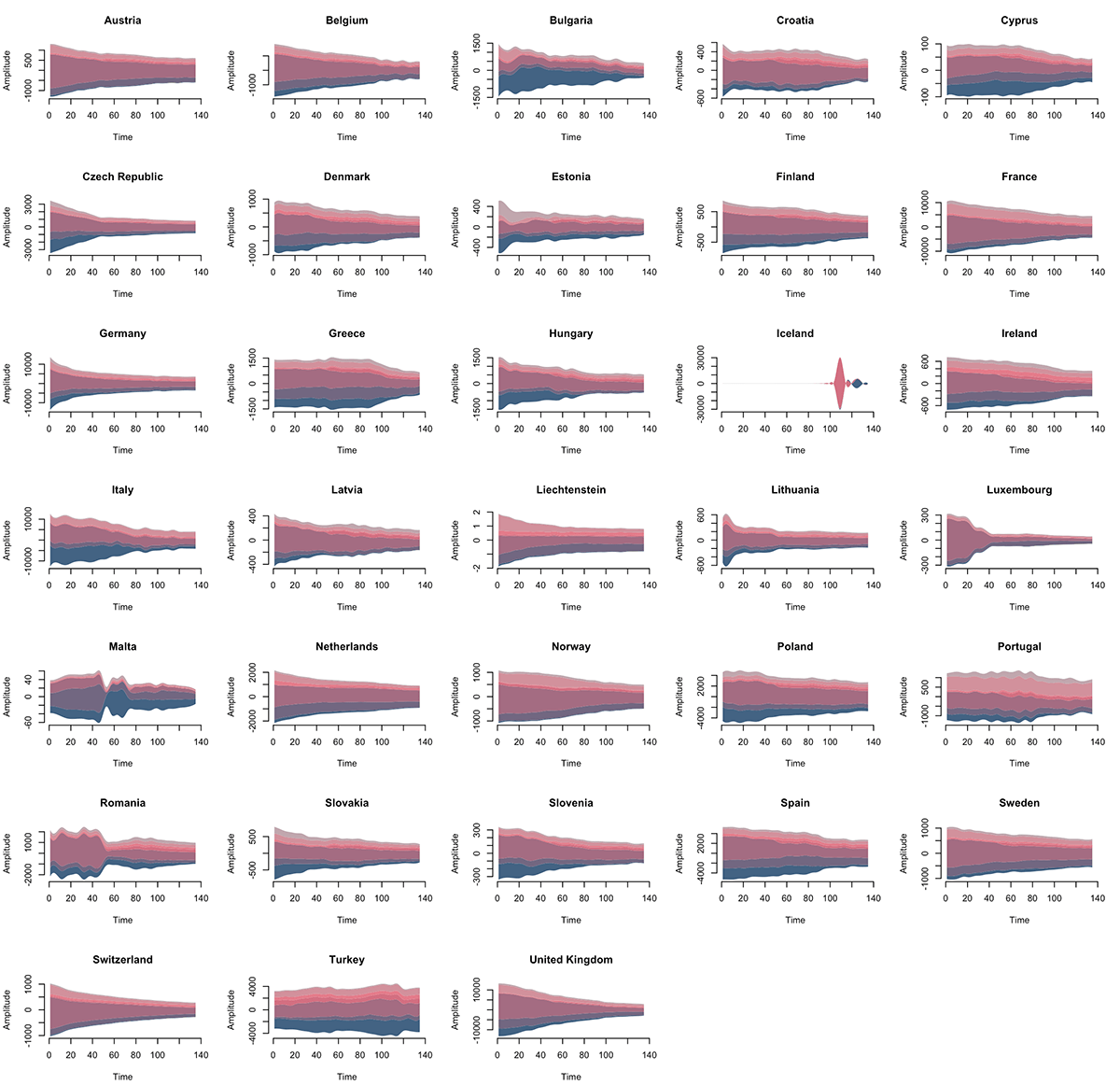
Making sure everything looks ok inside R:
Back to Tableau:
In Tableau the process is pretty much the same as before, only that we split the view by Rows and Columns.
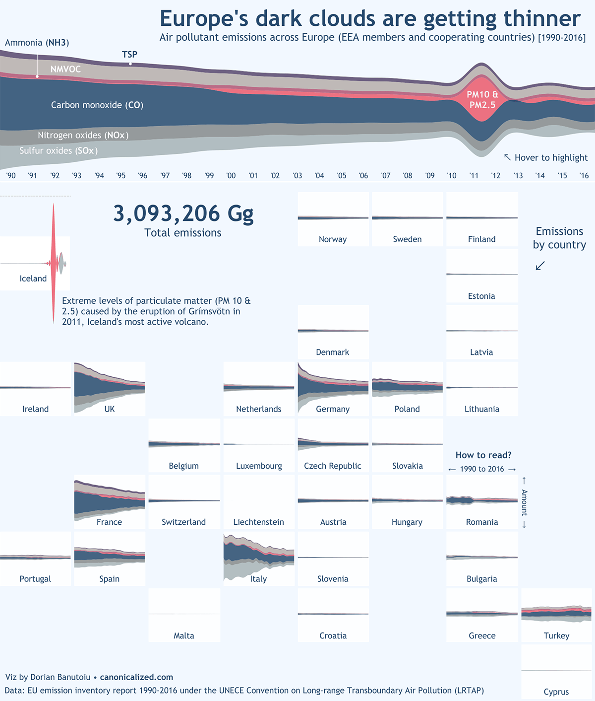
In our case, we even took it a step forward and matched the countries to their approximate geographic location.
Mic drop!
Examples of StreamGraph based dashboards in Tableau
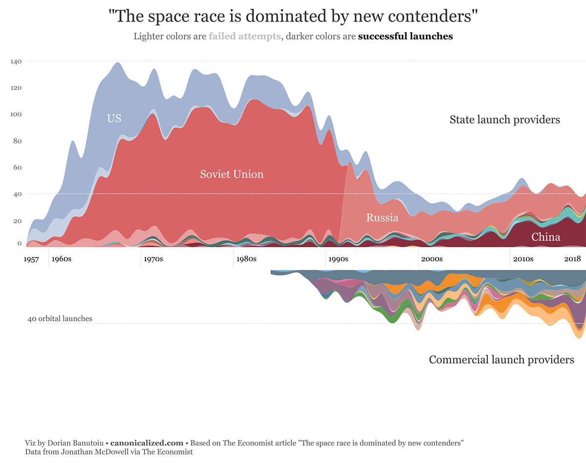
I want to share with you a couple of visualizations I built using this method. I think you will agree that they hold a strong visual effect.
(*click on the images to open up the interactive versions in Tableau Public)
Let me know if you have any feedback or if you need help figuring things out!
Update: the Space Race stream graph got featured as Viz of the Day on Tableau Public. A huge thanks to the community for making this possible!
Highly passionate about data, analysis, visualization, and everything that helps people make informed decisions.
I love what I do! I am working to improve speed in every aspect of my life and that of our clients.
I find comfort in helping people, so if you have a question, give me a shout!
